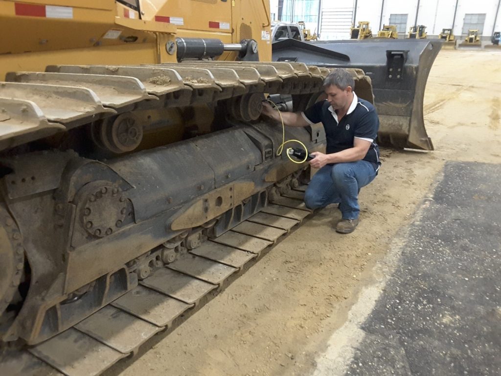
“It was only 75% worn at the last inspection. How did it wear out so quickly?” 

It’s a comment we hear regularly. An undercarriage component can wear slowly for thousands of hours, then go through the last of its usable wear material in a surprisingly short time. To understand why, it helps to look at what happens over the component’s whole life. 

An Expensive Consumable

So is an air filter. The difference is that you can buy a lot of air filters for the price of an undercarriage component.

Part of that cost comes from the hardening and other manufacturing processes used to resist wear. Furthermore, each component works as part of a larger system. Chains, sprockets, rollers, and idlers wear at different rates, and the aim is to manage that wear across the whole undercarriage. Regular inspections—as a result—and comparing the results from one inspection to the next, show whether that balance is being maintained.

Why wear speeds up towards the end 

The graph below shows an illustrative wear curve over an 8,000-hour useful life. The slope tells the story. It starts shallow, rises gradually through the middle and gets noticeably steeper towards the end. 

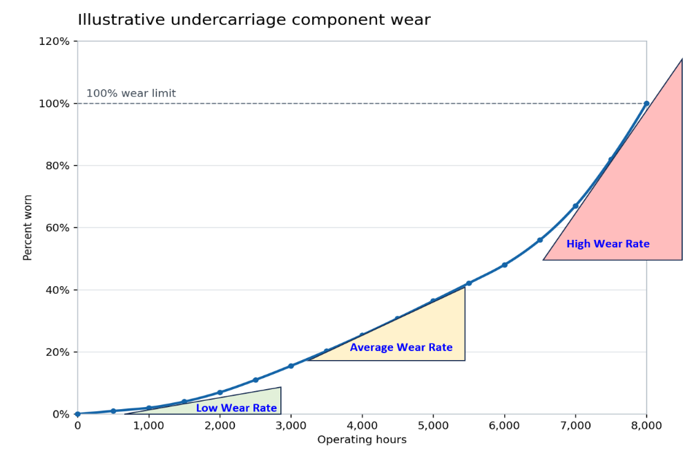
All undercarriage wear components are hardened in some way to resist wear. The method and depth of hardening varies by component. Where the working surface is harder than the material beneath it, wear is slow at first. As the component wears deeper into the material, the wear rate can increase. 

This is where an early forecast can get you into trouble. Take the percentage worn at an early inspection, divide the operating hours by that percentage, and project the result out to 100% worn. The arithmetic is straightforward. It also assumes the component will keep wearing at that same slow rate for its entire life. The graph shows how far that assumption can take you off course. 

Take this curve, for instance: at 2,000 hours, it reads about 7% worn. Divide and project, and you get a component that theoretically lasts 28,000 hours—when it actually fails at 8,000. Later on, at 75% worn, a simple straight-line forecast suggests you still have 2,400 hours left, whereas the actual curve shows closer to 700.

Towards the end of life, the opposite happens. The component can use up several percentage points of wear in a relatively short time. Each 1% of wear takes fewer operating hours than it did earlier in life. 

Use past performance to forecast what’s left 

A more effective starting point is the performance history of comparable components, where you compare the life of each component while considering the effects of seasonality, ground conditions, and machine application. From this history, you can determine an average wear rate expressed as operating hours per 1% of wear, or distance travelled per 1% of wear. In addition, reliability teams use this historical average wear rate alongside the latest inspection results and the shape of the wear curve to estimate how much life each component has left. As more comparable inspection history becomes available, you gain a better basis for refining the forecast.

For reliability engineers and asset managers, specifically, that means more time to plan replacements and get parts on site. Ultimately, it helps identify machines or components that consistently wear faster than expected and shows which components deliver the best life in a particular environment and application.